
A how to guide on linear regressions
A how to guide on linear regressions
The dog days of summer are almost over


We’ve been in the dog days of summer now for a few weeks, so it’s been hot. And on the east coast the heat and humidity means that even with the air conditioning on it can get a little toasty indoors. I live in a renovated older building, which has two units which double for heat and cooling, and recently, it’s been more than a little toasty. Working, sleeping, and cooking have all been activities I do not want to do. My solutions thus far have been a cold drink, an ice pack sitting in front of the unit, and retreating to the coffee shop down the street to get some cold air. Not great for morale. Luckily, my friend and neighbor recently moved and gave me his spare window AC unit. It’s been a godsend. Now the apartment is nice and cool even on the hottest days, and I can focus on preparing to be a TA for econometrics this fall. As I was preparing I realized it might be helpful to consolidate some modeling concepts into a post. Working with models all day can be difficult as you’ll see there is a lot to keep track of, but overall this post will hopefully either give you a better appreciation of attempting to create a model, or some advice for when your model doesn’t look very good.
Model? Who me? I could never!
The goal of a model is to have a guess based on a set of different information. Without realizing it we do this everyday— if you ever attempted to dress for the weather you considered a mental model of how hot you would feel based on an information set such as the temperature, humidity, cloud coverage, and then dressed accordingly.
Typically, this guess is for the “ideal” case. It follows that a “model” is for the ideal case- that under ordinary circumstances and given the available information then your prediction may be close to the reality you experience. For example, if you anticipate a 70 degF and rainy day, but it turns out to be 70 degF and a hurricane, your prediction may have been wrong and you may be in danger… the model wasn’t very helpful in this situation!
A model then might be helpful for 2 reasons:
To predict an ordinary future (which is impossible in the exact case but you might be better prepared for it if you have a guess)
To avoid data collection which can be costly
The first reason is reasonable- one might use a model to extrapolate polling data for example based on a limited set of survey data. This is easier than asking everyone who they will be voting for before heading to the polls.
The second reason may or not be useful. For example if the future is in fact ordinary, your prediction may turn out to be pretty close to reality. However, if you are under extraordinary circumstances (a pandemic, inflation, natural disaster, or a combination of all of them) you may be way off base anyway. In such an instance it may simply be better to be reactive to the shock than to try to predict it (which is impossible.)
Nevertheless, if you believe there is value in predicting the future (which I do!) there is a need to do it systematically. To do this is nontrivial, but possible.
The most basic model is as follows:
y = m*x + b
where variable y is meant to be forecasted from variable x according to some coefficient m and y intercept term b.
This simple relationship can work decently well for a pair (x and y) of correlated variables. It may even work well for a set of two variables called x1 and x2 to predict y. When multiple variables are used in a model like this, the form of the model is called multivariate regression instead of linear regression.

If one were to use a multivariate model, it would be bad practice to simply do the calculations and then look at the result without first considering the assumptions that come along with it. So, let’s do just that! What are the assumptions and how can you test / correct them if your model is in violation?
The uninterested reader might aim to skip the following technical paragraphs about some of the assumptions of a very common estimation method, called Ordinary Least Squares. I find it to be interesting and explain concepts in basic terms, however it is easy to get lost in the weeds.
Linearity
As the last line of the above graphic suggests, the relationship between x1 and y might not be a simple, direct, linear relationship. If it were a linear relationship, that means that an increase in x would vary directly with an increase in y. For example, if x1 increased by 1, y might increase by 2, but if x1 increased by 2 then we would expect y to increase by 4 (here the coefficient b0 would equal 2!) If this weren’t the case, another relationship between x1 and y might be established, for example x1^2 or x1^n where n is some other number.
To borrow an example from physics, kinetic energy varies with the square of velocity but varies directly with mass.
A statistical test to determine if linearity is the correct form of your model is called a Ramsey RESET test. In short this test compares adding additional polynomial terms to the model to see if it ends up being better. If it is, then likely either there is another form of the model you can use or there is an omitted variable which causes your coefficients to be biased, or deviate from their true value. Additionally, it may be the case that there was a structural break in the relationship over time. In this case, a Chow test or predictive failure test might be a good option.

Full rank
Formally, full rank is a term to describe a matrix meaning its columns are linearly independent. (I know that this sentence may not help)
Basically this equates to not having a repeat variable in your model. For example if the variable x1 is total revenue, x2 is quantity of goods sold, and x3 is average revenue (which is defined as total revenue divided by the number of goods sold) then you have a repeat variable. x3 depends on a combination of x2 and x1 so the coefficients on x1 and x2 might be different than the true value for the relationship. This problem, called multicollinearity, exists even if x3 is correlated with x2. It can be detected via the variance inflation factor and fixed by either adding a x2*x3 term or simply dropping x3.
Errors are roughly even
This means that your model over-predicts as much as it under-predicts. If your model consistently gave an overprediction, it would be straightforward to add a constant term to decrease all predictions until the point where the average error (defined as the difference between the predicted value and the actual value) was 0.

Additionally, if it were the case that errors were correlated with regressors, there may be an omitted variable or endogeneity (y depends on x which depends on y… a common problem in economics!) This type of problem may be tested with a Hausman test, and fixed with an instrument variable, which is correlated to the regressors but not correlated with the errors.
Homoscedasticity
Means that no matter what value x is, there is a relatively constant variance.
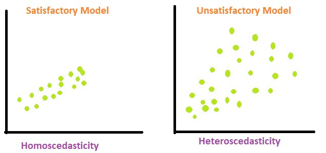
In the models above, the heteroscedastic model tends to vary more (the space between points) at larger values. Two ways to test for heteroscedasticity is through a GQ test and through a White’s test.
Non-autocorrelation
Meaning that you are likely to know the error of a point from the error of a previous point. You may find there is a pattern in the data around the trendline if there is either positive or negative autocorrelation. A Breusch-Godfrey test would test for for autocorrelation, and a lagged variable could be added as a remedy.

Errors are normally distributed
If there are “fat tails” in the distribution of errors plot, or equivalently, a data point(s) which is a large distance away from the trendline, it may disproportionately affect the regression and cause the coefficients to be different than the true value.

Given the white points in the above graph, the error term (so the difference between the white point and the trendline) follows roughly a normal distribution (the red curves). However, if the blue point is included, the new line of best fit (blue) shifts towards it and away from the original line of best fit. To test for this, one might use a Bera-Jarque normality test, and use dummy variables to avoid including the extreme values.
Relating this concept back to the top, the goal of the model is to predict “ordinary time.” The extraordinary event shouldn’t be included in the model since that isn’t the point of the model. The model itself wouldn’t be used under extraordinary times anyway (assuming there wasn’t measurement error causing the blue point to be off base.)
Conclusion
If any of the above assumptions are violated, then a simple linear model or multivariate model may not be the best one to use. But that doesn’t mean to give up!
For example, if you wanted to model something that counts, like the number of callers in an hour to a call center, or the number of goals throughout a soccer game, you might use a Poisson distribution.
Or if you’re modeling a time series, it might make sense to use an ARIMA model. (I made dashboard which teaches one how to create an ARIMA model here.)
Sometimes a simple linear model is a good place to start. It’s a way to think critically about what types of information might be important for a forecast and iterate from there. Just because your linear model isn’t working well doesn’t mean that the variable can’t be modeled. Sometimes you just need the right tool for the job. Sometimes an ice pack or a cold drink doesn’t cut it in a toasty older Philadelphia apartment, the right tool can make your job easier. And when it comes to forecasting, we need all the help we can get.
(Updated Sep 26, 2022)